import numpy as np
import matplotlib.pyplot as plt
from scipy.stats import multivariate_normal
def bivar(graphtype, mupos=None, sigpos=None, rhopos=None, muneg=None, signeg=None, rhoneg=None):
if mupos is None:
mupos = np.array([4, 4])
sigpos = np.array([1, 1])
rhopos = 0
muneg = np.array([2, 2])
sigmaneg = np.array([[1, -0.6], [-0.6, 1]])
else:
sigmapos = np.array([[sigpos[0], rhopos * np.sqrt(sigpos[0] * sigpos[1])],
[rhopos * np.sqrt(sigpos[0] * sigpos[1]), sigpos[1]]])
if signeg is None:
sigmaneg = np.array([[1, -0.6], [-0.6, 1]])
else:
sigmaneg = signeg
Npos = 100
Nneg = 100
pos = np.random.multivariate_normal(mupos, sigmapos, Npos)
neg = np.random.multivariate_normal(muneg, sigmaneg, Nneg)
mn = np.min(np.concatenate((pos, neg), axis=0))
mx = np.max(np.concatenate((pos, neg), axis=0))
x = np.arange(mn, mx, 0.1)
y = np.arange(mn, mx, 0.1)
X, Y = np.meshgrid(x, y)
Ppos = np.zeros_like(X)
Pneg = np.zeros_like(X)
L = np.zeros_like(X)
for i in range(len(x)):
for j in range(len(y)):
Ppos[j, i] = getprob(x[i], y[j], mupos, sigmapos)
Pneg[j, i] = getprob(x[i], y[j], muneg, sigmaneg)
L[j, i] = Pneg[j, i] / Ppos[j, i]
Pb = (1 / (2 * np.pi * np.sqrt(np.linalg.det(sigmapos)))) * np.exp(-1 / 2)
Ps = (1 / (2 * np.pi * np.sqrt(np.linalg.det(sigmaneg)))) * np.exp(-1 / 2)
plt.figure(figsize=(8, 8))
if graphtype == 2:
plt.axis('square')
plt.axis([mn, mx, mn, mx])
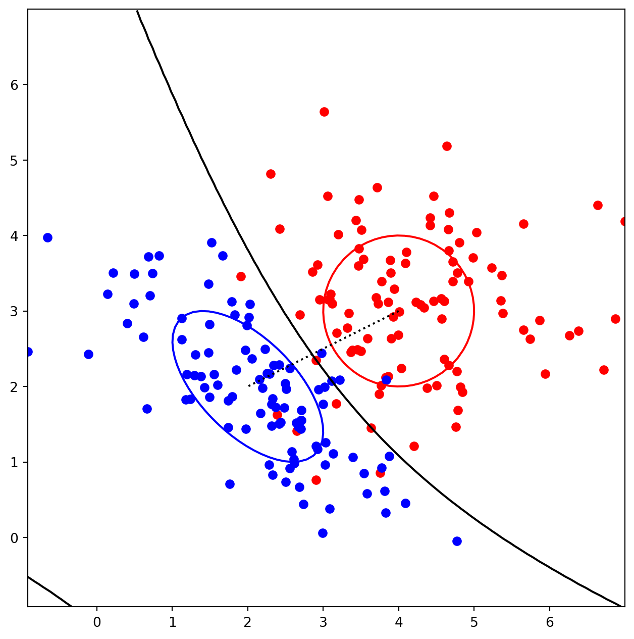
plt.scatter(pos[:, 0], pos[:, 1], color='r', label='Positive')
plt.scatter(neg[:, 0], neg[:, 1], color='b', label='Negative')
plt.contour(X, Y, Ppos, levels=[Pb], colors='r')
plt.contour(X, Y, Pneg, levels=[Ps], colors='b')
plt.contour(X, Y, L, levels=[1], colors='k')
plt.plot([mupos[0], muneg[0]], [mupos[1], muneg[1]], color='k', linestyle=':')
elif graphtype == 3:
from mpl_toolkits.mplot3d import Axes3D
fig = plt.figure(figsize=(8, 8))
ax = fig.add_subplot(111, projection='3d')
ax.plot_surface(X, Y, Ppos, cmap='Reds', edgecolor='none', alpha=0.6)
ax.plot_surface(X, Y, Pneg, cmap='Blues', edgecolor='none', alpha=0.6)
ax.contour3D(X, Y, Ppos, levels=[Pb], cmap='Reds')
ax.contour3D(X, Y, Pneg, levels=[Ps], cmap='Blues')
plt.show()
def getprob(x, y, mu, sigma):
vec = np.array([x, y])
E = 2 * np.pi * np.sqrt(np.linalg.det(sigma))
P = (1 / E) * np.exp(-0.5 * np.dot(np.dot((vec - mu), np.linalg.inv(sigma)), (vec - mu).T))
return P
bivar(2, mupos=[4, 3], sigpos=[1, 1], rhopos=0, muneg=[2, 2], signeg=[[1, -0.6], [-0.6, 1]], rhoneg=0)